ON THE ART AND SCIENCE OF ACOUSTIC INSTRUMENTS
© 2000–2025 Cris Forster
CHAPTER 8: SIMPLE FLUTES
Part I: Equations for the Placement of Tone Holes on Concert Flutes and Simple Flutes
Flutes, harps, and drums are the oldest musical instruments created by man. Wind instruments are unique, however, because they alone embody the physical dimensions of scales and tunings. In a work entitled The Greek Aulos, Kathleen Schlesinger (1862–1953) attempted to reconstruct Greek music theory by analyzing the remains of ancient reed flutes.[1] It is possible to approach the subject of flute tunings from two different perspectives. We may predict the tuning of an existing instrument by first measuring various flute bore, embouchure hole, and tone hole dimensions, and then substituting these data into a sequence of equations. This method provides convenient solutions when a flute is extremely fragile and cannot be played, or is simply not available for playing. On the other hand, we may realize a given tuning by making a flute according to another sequence of equations. From a mathematical perspective, these two approaches are distinctly different and require separate discussions.
As all experienced flute players know, the intonation of a transverse flute — with either a very simple or a very complex embouchure hole — depends not only on the precision of instrument construction, but also on the performer. The mathematics of flute tubes, embouchure holes, and tone holes does not necessarily produce an accurate sounding instrument. The intonation of a flute is also governed by the strength of the airstream, and by the amount the lips cover the embouchure hole. Because these two variables exist beyond the realm of mathematical predictability, they depend exclusively on the skill of the performer.
Due to the overall complexity of flutes, this chapter is divided into three parts. Part I investigates equations for the placement of tone holes, and Part II, mathematical procedures required to analyze existing flutes. Since Part II is unintelligible without a thorough understanding of Part I, the reader should study this chapter from beginning to end. Finally, Part III gives some suggestions on how to make very inexpensive yet highly accurate simple flutes.
Section 8.1
In writing this chapter, I am indebted to Cornelis J. Nederveen. In his book entitled Acoustical Aspects of Woodwind Instruments,[2] Nederveen carefully defines all the mathematical variables needed for a thorough investigation into woodwind acoustics. Numerous tables of woodwind instrument dimensions are included at the end of the book. Because a full description of flute acoustics requires many different variables, this discussion begins with a list of symbols originally defined by Nederveen. Since most of these symbols appear only in this chapter, they are not included in the List of Symbols at the beginning of this book. Furthermore, the List of Flute Symbols below gives seven symbols that do not appear in Nederveen’s book: effective length LB(h) replaces λH; effective length LB(e) replaces λE; correction ΔlE replaces LB(e) in the context of flute length calculations; corrections ΔlH and ΔlT, and length lT, represent simplifications. Finally, LA replaces LS when, in predicting the frequencies of an existing flute, we cannot determine LS, which represents an exact acoustic half-wavelength; in this context, we must calculate LA, which represents an approximate acoustic half-wavelength. In preparation for Chapter 8, the reader should read, study, and absorb Chapter 7. Knowledge of longitudinal pressure waves and end correction terminology is essential for an understanding of flute acoustics.
Recall that in Chapter 7, Section 12, we discussed the great convenience of centimeter measurements for cutting resonator lengths. A similar advantage also applies to flute construction. However, because many flute dimensions are much smaller than resonator dimensions, we will use millimeter measurements throughout this chapter. To convert inches to millimeters, multiply inches by 25.40; and to convert millimeters to inches, multiply millimeters by 0.039370.[3]
Finally, we must also define a dimensionally consistent speed of sound (c) inside a flute. Heat, water vapor, and carbon dioxide from the player’s breath, as well as mechanical boundary layer effects that are frequency sensitive, all affect the value of c.[4] For simplicity, assume an average temperature of 25°C (or 77°F) inside the flute, and not accounting for changes due to frequency,[5] we will therefore use c = 346,000 mm/s in all future calculations.[6]
Section 8.2
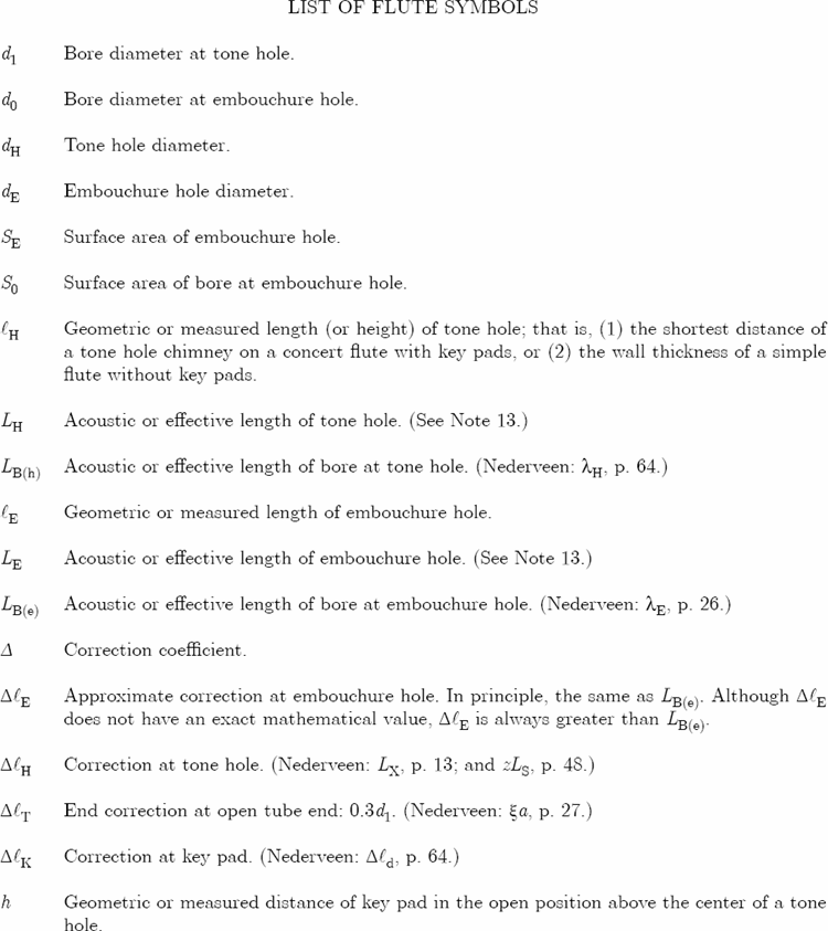
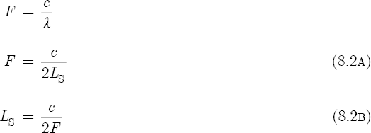
We begin this discussion on the mathematics of flute construction by carefully distinguishing between a tube’s invisible acoustic length and its visible geometric length. Figure 8.1 shows that for the fundamental mode of vibration, the acoustic length of a tube open at both ends spans the distance of a half-wavelength. Similarly, Chapter 7, Figures 12(a) and 12(b), show that the acoustic length of a resonator closed at one end spans the distance of a quarter-wavelength. The latter three figures illustrate that a tube’s acoustic or effective length (Leff) is slightly longer than its geometric or measured length (L). In this context, the acoustic length is of paramount importance because it alone determines a tube’s fundamental wavelength (λ1). For a tube open at both ends, λ1 = 2Lo eff. (See Equations 7.22 and 7.24.) And for a tube closed at one end, λ1 = 4Lc eff. (See Equations 7.27 and 7.29.)
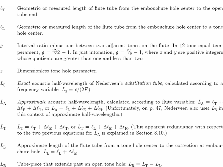
Until now, we have not considered tubes closed at both ends because they serve no practical musical purpose. However, such tubes are fundamentally important because they provide a theoretical basis for flute length calculations. Figure 8.2 shows a tube closed at both ends, also called a closed-closed tube. For a closed-closed tube, the distinction between an acoustic/effective length and a geometric/measured length does not exist. Since there are no openings, pressure waves or displacement waves inside the tube do not reflect a small distance beyond the tube’s physical length. Instead, all waves reflect precisely at the tube’s closed ends.Consequently, end corrections are not a factor,[7] which means that for a tube closed at both ends, λ1 = 2Lclosed-closed. The equation for the theoretical and actual fundamental frequency (F1) of a closed-closed tube states
![]()
where L is the tube’s inner measured length.
Nederveen refers to a closed-closed tube as a substitution tube, and notates its inner geometric length, L or its exact acoustic half-wavelength, as LS.[8] Since the acoustic and geometric lengths are identical, we now set LS = L. Substitute LS into Equation 8.1 and solve for the acoustic half-wavelength in the following manner:[9]
A transverse flute consists of a tube open at both ends. The embouchure hole provides the first opening, and the far end of the flute, or an open tone hole, provides the second opening. Turn to Figures 8.3(a), 8.3(b), and 8.3(c), and observe that each illustration consists of two sections. The top portion shows a substitution tube closed at both ends, and the bottom portion shows a flute tube open at both ends. Nederveen’s substitution tube exemplifies a tube without any openings that generates exactly the same frequency as a flute tube with two openings.[10] Stated another way, LS represents the acoustic half-wavelength that a flute tube produces when it sounds a given frequency. Therefore, we now write the following condition for the purposes of flute length calculations:
This expression states that the acoustic/geometric length of a substitution tube, or of a tube closed at both ends, is by definition identical to the acoustic/effective length of a tube open at both ends.
Due to the reflection of waves a small distance beyond the flute openings, the geometric/measured length from the embouchure hole center to the open tube end (lT), and the geometric/measured length from the embouchure hole center to a tone hole center (lL), are always shorter than LS. Figure 8.3(a) shows that lT is shorter than LS because of an added embouchure correction (ΔlE) at the top or high end, and an added end correction (ΔlT) at the bottom or low end. Similarly, Figures 8.3(b) and 8.3(c) show that lL is also shorter than LS because of ΔlE at the top end, and a tone hole correction (ΔlH) past the tone hole center at the bottom end.
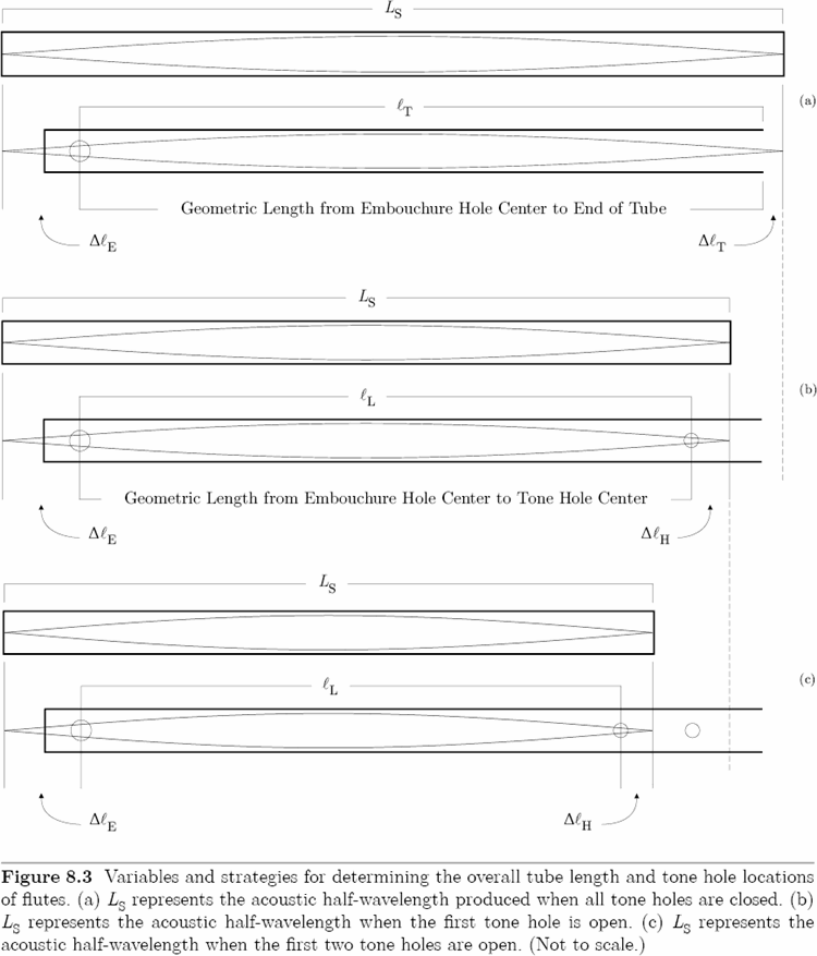
Since the lT and lL length dimensions determine in large part the tuning of a flute, we will compute these variables in the following manner. (1) For the flute’s lowest tube frequency when all tone holes are closed, evaluate Equation 8.2b and then replace LS with LS(t); and for all higher frequencies when one or more tone holes are open, again evaluate Equation 8.2b and then replace LS with LS(h). (2) Next, calculate the corrections ΔlE, ΔlT, and ΔlH. (3) Finally, determine lT by subtracting ΔlE and ΔlT from LS(t),
![]()
and (4) determine lL by subtracting ΔlE and ΔlH from LS(h):
![]()
In Section 8.3, a solution to Equation 8.3 for a concert flute with keys predicts lT within 3.5 mm (0.138 in.) of the measured length. And in Section 8.6, twelve solutions to Equation 8.4 for the same concert flute predict lL within 1 mm (0.039 in.) of the measured lengths.
Before we continue, it is important to first clear up a semantic problem. In Section 8.1, the List of Symbols defines four corrections: ΔlE, ΔlH, ΔlT, and ΔlK. The last two corrections have simple, straightforward solutions. However, as explained in Sections 8.3 and 8.5, the first two corrections are more complicated because they are derived from proportions. The List of Symbols carefully defines ΔlE as a “correction at the embouchure hole.” It does not define ΔlE as an “embouchure hole correction.” The latter definition suggests that ΔlE is a sole function of the embouchure hole. This is not the case. Section 8.3 explains that ΔlE has its origins in the following proportion:
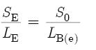
where S0 is the surface area of the bore at the location of the embouchure hole, and LB(e) is the effective length of the bore at the location of the embouchure hole. At the end of Section 8.3, we will replace LB(e) with ΔlE. This example demonstrates why it is technically more accurate to call ΔlE a “correction at the embouchure hole” than to give the impression that ΔlE is an “embouchure hole correction.” However, phrases like “the correction at the embouchure hole” and “the correction at a tone hole” are awkward in the context of a difficult discussion. Therefore, we will continue to use the phrases “embouchure hole correction” and “tone hole correction” even though such expressions do not give exactly correct descriptions.
Section 8.3
We turn our attention now to solutions for ΔlT and ΔlE. Chapter 7, Section 11, discussed at length the end correction phenomenon that occurs at the open ends of cylindrical resonators. Since the end correction for a flute tube is the same as for a resonator tube, refer to Equation 7.20, set ΔlT = Δl, and use this equation for the end correction:
![]()
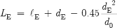
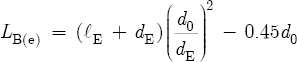
Unfortunately, an exact equation for the embouchure correction does not exist. ΔlE depends on the position of the player’s lips over the embouchure hole. Increased lip coverage increases ΔlE.[11] This causes an increase in LS (see Equation 8.20), which in turn decreases the frequencies of the flute. However, Nederveen does give a solution for the minimum theoretical value[12] for the effective length of the bore at the embouchure hole,[13]

where lE is the measured length or height of the embouchure hole, in millimeters; dE is the diameter of the embouchure hole, in millimeters; and d0 is the diameter of the flute bore at the location of the embouchure hole, also in millimeters.
To understand the origins of Equation 8.6, we must first consider the acoustic admittance (YA) of a flute bore or flute hole. This quantity measures the ease with which air flows through a duct. Acoustic admittance is the reciprocal (or opposite) of acoustic impedance:[14]

As the impedance of a duct increases, the admittance decreases; vice versa. A non-complex definition[15] of acoustic impedance is
![]()
Therefore, a non-complex definition of acoustic admittance is

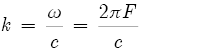
where S is the surface area of the duct, in square millimeters; ρ is the density of air, in kilograms per cubic millimeters; c is the speed of sound, in millimeters per second; k (Lat.) is the angular wave number,[16] in radians per millimeter; and κ (Gk.) is the conductivity of the hole, in millimeters. Conductivity is the reciprocal (or opposite) of resistance. We define conductivity as the ratio of a duct’s surface area divided by its effective length[17]

where S is the surface area of a bore or hole, in square millimeters; l is the measured length of a bore or hole, in millimeters; d is the diameter of a bore or hole, also in millimeters; and Δ is the correction coefficient of a bore or hole,[18] dimensionless. Equation 8.9 states that the airflow through a hole is directly proportional to surface area, and inversely proportional to effective length. A wide shallow hole conducts air more efficiently than a narrow deep hole. Note, however, when κ is too large or too small for a given bore, the flute tube is either too long or too short and will not work. Similarly, when κ is too small for a given tone hole, the hole is too narrow and will not work. Equations 8.7 and 8.8 show that ZA and YA are functions of conductivity. For a given bore or hole, the ratio of S to l + Δ(d) must be correct, otherwise the terminating admittance (or terminating impedance) will not cause a reflection of pressure waves from the openings of a bore, nor from the opening of a hole.[19] Without the reflection of pressure waves, there can be no standing waves, and without standing waves, there is no sound.
Consider now the locations on a flute where two admittances (of conductivities κ) are simultaneously present. Such a place exists at the top end of the flute. Here the conductivity of the embouchure hole interacts with the conductivity of the flute bore at the location of the embouchure hole. The flute provides us with the dimensions of the diameter and the length of the embouchure hole, and the diameter of the bore. However, because the effective length of the bore at the location of the embouchure hole remains unknown, we may solve for LB(e) by considering the following proportion. Equation 8.10 states that the surface area of the embouchure hole (SE) is to the effective length of the embouchure hole (LE), as the surface area of the main bore at the embouchure hole (S0) is to LB(e):
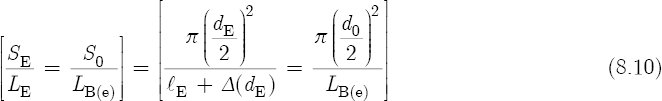
To solve for LB(e), cross-multiply, divide, cancel, and simplify:
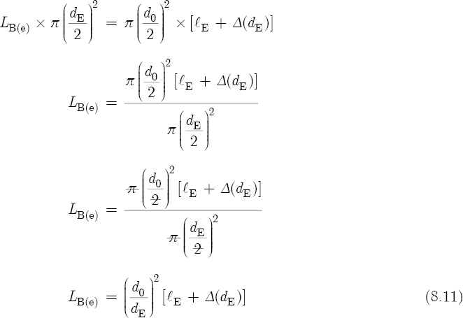
Equation 8.10 defines the conductivity of one duct in terms of another duct. The difference between these two ducts is that the left side of Equation 8.10 represents the actual duct of the embouchure hole, whereas the right side of Equation 8.10 represents a fictitious duct associated with the bore. This fictitious duct has the same diameter as the flute tube, and by definition, the same conductivity as the embouchure hole. Figures 8.3(a), 8.3(b), and 8.3(c) show that LB(e) (or ΔlE) of the fictitious duct has the effect of extending the bore beyond the top end of the flute. Equation 8.10 states that the actual and the fictitious ducts must have the same conductivity, otherwise two different admittances would result. If two different admittances existed, then the pressure waves would not reflect from the same location to the left of the bore. We conclude, therefore, that for a given frequency, the combined terminating admittances of the embouchure hole and the bore cause a reflection of pressure waves a moderate distance LB(e) beyond the physical location of the embouchure hole center. Similarly, recall that in Chapter 7, Section 11, the impedance of a resonator causes a reflection of pressure waves a small distance Δl beyond the physical length of the tube.
According to Arthur H. Benade,[20] a good estimate for the coefficient of both the inside and outside corrections[21] of an embouchure hole or tone hole is Δ = 0.75. To ensure that the results of Equations 8.6 and 8.11 are very close, we will use a slightly smaller correction coefficient, Δ = 0.71. Consider now the following embouchure and bore dimensions of a typical concert metal flute:
lE = 4.3 mm. Due to the presence of a lip plate, the length of the embouchure hole is much greater than the thickness of the flute tube; the wall of a typical concert flute is only 0.5 mm thick.
dE = 11.2 mm. On most concert flutes the embouchure hole is in the shape of an oval and has a diameter of 12 mm; here 11.2 mm represents a mean value.[22]
d0 = 17.4 mm. The embouchure end of a concert flute — also known as the head joint — has a slight taper that decreases the tube’s diameter from 19.0 mm at the joint to approximately 16.8 mm at the far upper end of the tube.
A substitution of these values into Equation 8.6 gives LB(e) = 29.58 mm, and into Equation 8.11 gives LB(e) = 29.57 mm.
Four years after the publication of his book, Nederveen concluded that empirical observations over a wide frequency range indicate LB(e) ≈ 50 mm.[23] Theobald Boehm[24] (1794–1881), the inventor of the modern concert flute, and Benade give the same approximation. Since the effective length of the bore at the embouchure hole acts as a correction, express the following condition for the purposes of flute length calculations:
![]()
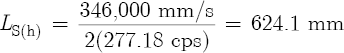
and assign the value ΔlE = 50 mm. Now, to calculate lT for a concert flute tuned to middle C (or C4 at 261.63 cps), first use Equation 8.2b to compute the acoustic length of the substitution tube:
Next, substitute a 19.0 mm diameter bore into Equation 8.5 to obtain the end correction:
![]()
Finally, substitute the values for LS(t), ΔlE, and ΔlT into Equation 8.3 to obtain the tube length:
![]()
Section 8.4
On the Armstrong Concert Flute (Serial Number 104-25-29992), lT = 602 mm, which is 3.5 mm shorter than given by the previous calculation. To account for this shorter length, we must examine the profile of a flute bore in greater detail. While playing the lowest frequency, a flute bore does not have a perfectly smooth surface. Instead, a series of closed tone holes gives the bore an interrupted and irregular profile. Closed tone hole cavities have the effect of enlarging the volume of the bore and perturbing the flow of air through the bore.[25] This causes the flute to sound flat. Furthermore, the viscous and thermal losses associated with a thin boundary layer against the flute’s inner surface, and the shape of the tapered head joint at the top end of the flute, also effectively decrease the frequencies of a flute throughout the first “octave” of its three “octave” range. For a Gemeinhardt Concert Flute,[26] which is very similar to the Armstrong Concert Flute, Nederveen shows that these combined corrections cause the flute to sound C4 between 15–30 ¢ flat. To help offset these effects, flute makers intentionally shorten lT by a small amount. According to Equation 8.1, as lT or L decreases, λ1 decreases, and so F1 increases. Although a 3.5 mm shorter length for this flute sounds F1 only 9.2 ¢ higher, the performer’s blowing technique at the embouchure hole corrects any remaining intonational discrepancies.
During the early stages of making a simple flute, mark the location of the embouchure hole 32 mm (1 1/4 in.) from the upper end of the tube; now cut the tube 10 mm longer than given by Equation 8.3. Drill the embouchure hole, and place a cork into the tube so that the cork’s inner surface sits 17 mm to the left of the embouchure hole center. (In concert flutes, 17.0 mm is the standard distance between the embouchure hole center and cork.) Test the frequency of the tube without tone holes. Gradually shorten the tube until it gives a frequency about 30 ¢ flat of the fundamental frequency. Stop for now. For the embouchure hole correction use ΔlE = 52 mm (see Section 8.7), and calculate the tone hole locations as specified in Section 8.5. Drill the tone holes with a small diameter drill at first: this causes all the holes to sound flat. Fine-tune the flute by gradually enlarging the tone hole diameters: this raises the frequencies. Intermittently test the lowest frequency of the flute with all tone holes closed. Finally, fine-tune the flute bore by gradually decreasing the length of the tube. As lT decreases, F1 increases and comes into tune.
Section 8.5
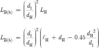
Our next task is to calculate the tone hole correction. On first impression, Figure 8.3(b) seems to suggest that ΔlE and ΔlH represent equivalent quantities. This is not the case. Equation 8.17 and Equation 8.18 show that ΔlH is a function of the effective length of the bore at the location of a tone hole (LB(h)). Unlike LB(e), LB(h) has a predictable value because it does not depend on the technique of the flute player. Analogous to LB(e), LB(h) represents the length of a fictitious duct that has the same diameter as the main tube, and the same conductivity as the tone hole. However, LB(h) alone does not define ΔlH. With respect to LB(e), the flute tube ends near the embouchure hole. But with respect to LB(h), the flute tube does not end near the open tone hole. Instead, pressure waves continue to travel inside the bore beyond the physical location of the open tone hole. For this reason, we must also account for the terminating admittance of the short tube-piece that extends past the open hole. For the first tone hole in Figure 8.3(b), the effective length of this tube-piece spans the distance from the tone hole center to the dashed line. This line marks the end correction at the open end of the tube. Similarly, in the case of two adjacent open holes, the effective length of the tube-piece in Figure 8.3(c) spans the distance from the second tone hole center to the dashed line. Here the line marks the tone hole correction of the first tone hole. We conclude, therefore, that ΔlH is a function of three admittances. For a given frequency, the combined terminating admittances of the tone hole, the flute bore, and the tube-piece cause the reflection of pressure waves a moderate distance ΔlH beyond the physical location of the tone hole center.[27]
Before proceeding with detailed calculations, let us first distinguish between flutes with key pads, and those without key pads. A key pad has the effect of decreasing the frequency of a tone hole. Consequently, a tone hole with a key pad sits higher on the bore (or nearer the embouchure hole) than a tone hole without a key pad, which sits lower on the bore (or nearer the flute’s open end). For a tone hole with a key pad, the higher position compensates for this flattening effect and, thereby, increases the frequency of the hole. Since most modern concert flutes come equipped with key pads, we continue our analysis of the previously mentioned concert flute.
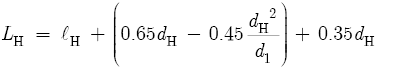
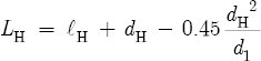
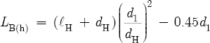
For a flute with key pads, ΔlH requires preliminary solutions to Equations 8.2B, 8.12, 8.13, 8.16, and 8.17; and for a flute without key pads, ΔlH requires solutions to Equations 8.2B, 8.14, 8.16, and 8.17. Nederveen gives the following equation for the effective length of the bore at the location of a tone hole:[28]

where lH is the shortest distance of a tone hole chimney,[29] in millimeters; dH is the diameter of the tone hole, in millimeters; ΔlK is the key pad correction, in millimeters; and d1 is the diameter of the bore, also in millimeters. With the exception of the ΔlK variable, notice the similarities between Equations 8.6 and 8.12. Nederveen and Benade give[30]
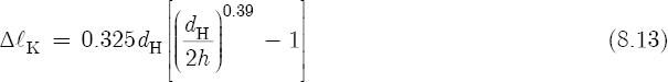
where h is the key pad distance in an open position above the center of the tone hole, in millimeters. Remember, however, that for a simple flute without key pads, we must rewrite Equation 8.12 without the ΔlK variable:
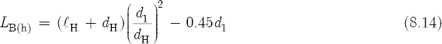
Equation 8.14 suggests that the proportion expressed by Equation 8.10 applies not only to embouchure holes, but to tone holes as well. Consequently, Equation 8.15 also gives good results:

Consider now the following C#4 tone hole dimensions, key pad and bore dimensions, and key pad correction of the same concert flute:
A substitution of these values into Equation 8.12 gives LB(h) = 21.5 mm, and into Equation 8.15 gives 22.0 mm.
To determine ΔlH, we must also consider a musical interval or the interval ratio between two adjacent tone holes on the flute. In this context, Nederveen gives this variable,[31]
![]()
where x/y is either a rational or irrational interval ratio. For a scale in 12-tone equal temperament,[32] where all the intervals between adjacent tones are constant, g equals the 12th root of 2 minus one:
![]()
However, for a scale in just intonation,[33] g is not necessarily a constant. For example, if the first tone hole is a 9/8, or a “just major second,” then the interval ratio between the lowest frequency of the flute tube and the first hole is a 9/8,
![]()
and so,
![]()
But if the second tone hole is a 5/4, or a “just major third,” then the interval ratio between the first hole and the second hole is a 10/9,
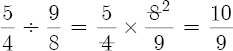
and so,
![]()
Nederveen combines variables LB(h), g, and LS into a dimensionless tone hole parameter:[34]
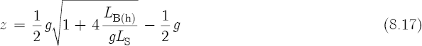
According to Equation 8.2b, for the first C#4 tone hole
so that,
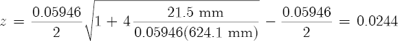
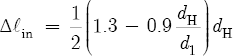
Finally, Nederveen gives the tone hole correction[35]
![]()
so that,
![]()
For the location of the C#4 tone hole, substitute the values for LS(h), ΔlE, and ΔlH into Equation 8.4 to obtain the tube length:
![]()
This corresponds to the exact location of the first hole on the concert flute.
Section 8.6
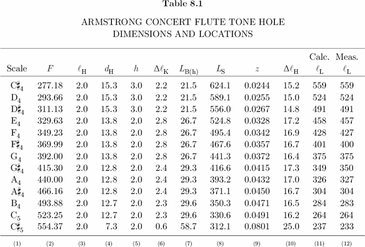
Table 8.1, Columns 3–5, list tone hole and key pad dimensions of the Armstrong Concert Flute, and Columns 6–10 list the results of five equations required to compute lL. Finally, Column 11 gives the calculated tone hole locations, and Column 12 gives the measured tone hole locations, rounded here to the nearest millimeter. With the exception of the C#5 tone hole, there is very good agreement between calculated and measured locations. The C#5 hole also serves as a vent or register hole for D5 and D#5.[36] Its location is designed to correct the lengthening (or flattening) effect of the tapered head joint.[37] For this reason, the C#5 hole has a comparatively small diameter and sits 3.5 millimeters higher on the bore than predicted by theory.
Section 8.7
One of the most important relations to emerge from Table 8.1 is that lL is directly proportional to dH:
![]()
As the diameter of a tone hole decreases, the distance from the embouchure hole center to a tone hole center decreases as well; vice versa. For a given frequency, a small diameter hole sits higher on the bore than a large diameter hole. For example, if we decrease the diameter of the C#4 hole in Table 8.1 to 14.3 mm, then lL = 558 mm, which means that this smaller hole would have a position 1 mm higher on the bore than the existing hole. This is an important consideration for makers of simple keyless flutes. The usefulness of a simple flute depends in large part on the spaces between tone holes, because if the tone holes are too difficult to reach, the instrument is unplayable.
Most simple flutes consist of an embouchure hole and six tone holes. One plays the fundamental by closing all the holes, then six more tones by opening each hole, and finally the eighth tone, or the “octave,” by closing all the holes again and overblowing at the embouchure hole.[38] Consider such a flute tuned to G4 at 392.0 cps. To play a just intoned diatonic scale on this instrument requires six tones holes that produce the following six frequency ratios and six interval ratios:[39]
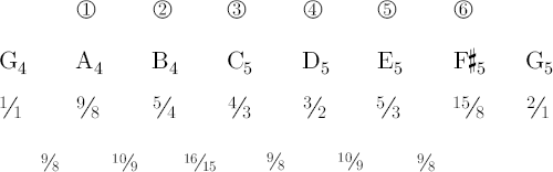
Between 15/8 and 2/1, we do not include the last interval, ratio 16/15, because it occurs naturally while overblowing the flute.
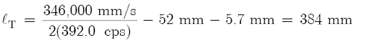
Table 8.2(a) lists tone hole dimensions and solutions for such a flute tuned to 392.0 cps., where d1 = 19.0 mm (3/4 in.), lH = 3.2 mm (1/8 in.), and lT = 384 mm (15.1 in.). The latter value results when we substitute ΔlE = 52 mm into Equation 8.3:
The embouchure hole has the following dimensions: d0 = 19.0 mm, lE = 3.2 mm, and dE = 9.5 mm (3/8 in.). Substitute these values into Equation 8.6 and calculate LB(e) = 42.3 mm. Tests show that for such a cylindrical flute with a simple circular embouchure hole, and without a tapered head joint,[40] ΔlE = 52 mm. This actual correction is typically between 9–10 mm greater than the theoretical correction, and 2.0 mm greater than the empirical correction of a standard concert flute. Such conclusions are based not only on experimental observation, but also on personal preference. Equation 8.4 shows that ΔlE plays a critical role in determining the locations of all tone holes. That is, as ΔlE increases, lL decreases, which means that a higher value for ΔlE places all the tone holes closer to the top end of the flute. Since lL is inversely proportional to F (see Section 8.8), as lL decreases, F increases. Note, however, that the intonation of a tone hole depends not only on location, but also on the strength of a player’s airstream, and on the lip coverage of the embouchure hole. A weak airstream and a large lip coverage tend to flatten (or decrease), and a strong airstream and a small lip coverage tend to sharpen (or increase) all the tones of a flute. Consequently, when a series of tone holes sits 2.0 mm higher on the bore, the player is more relaxed because high tone hole locations require less air pressure and allow more lip coverage without the risk of sounding flat. On the other hand, if the player chooses to play loud, or play in the second or third registers, the flute requires greater air pressure and less lip coverage, two conditions that tend to sharpen all the tones. These potentially conflicting relations indicate that there are no hard rules governing ΔlE. The final value of the embouchure correction is (within limits) subject to the discretion of the flute maker.
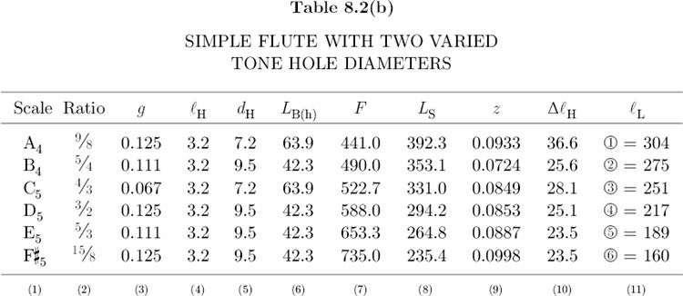
We return now to Table 8.2(a) where Column 7 gives the frequencies of the tone holes in just intonation. To calculate these frequencies, multiply 392.0 cps by a given frequency ratio. For example, frequency of F#5 is 392.0 cps × 15/8 = 735.0 cps. (As before, use c = 346,000 mm/s to calculate LS.) For all holes dH = 9.5 mm (3/8 in.). Notice that the space between holes z and x is 38 mm, and between holes x and c is 17 mm, which constitutes an irregular spacing, but between holes v and n it is 28 mm, and between n and m it is 29 mm, which constitutes a regular spacing. The irregular spacing of the first three holes is due in large part to the semitone between B4 and C5. If we decrease the diameters of holes z and c to dH = 6.4 mm (1/4 in.), then lL for z = 299 mm, and for c = 248 mm, so that both holes would occupy higher locations on the bore. Now the spacing between holes z and x would be 24 mm, and between holes x and c would be 27 mm. This is a much more comfortable design. The only drawback for such small diameter holes is that the surface areas are also smaller. According to Equation 8.7, as S decreases, ZA increases, which means that smaller holes have a higher wave impedance and, therefore, radiate acoustic energy less efficiently than large holes.[41] Consequently, for a given blowing pressure, small holes are not as loud as large holes. This discrepancy between 9.5 mm holes and 6.4 mm holes in the lower part of the bore is rather noticeable. However, Table 8.2(b) shows that if we decrease the diameters of holes z and c from the original 9.5 mm to 7.2 mm (9/32 in.), then the space between holes z and x is 29 mm, and between holes x and c is 24 mm. Although a 9/32 in. hole is only 1/32 in. larger than a 1/4 in. hole, the difference in amplitude is strikingly perceptible and very similar to the amplitude of a large 3/8 in. hole. Note that the new spacing between the lower three holes also represents a well-balanced design. In Plate 11, the flute on the left — or Flute 1 — has the dimensions and tuning of this flute described in Table 8.2(b). (See Instruments and Music > Simple Flutes.)

Section 8.8
In conclusion to Part I, let us continue the discussion begun in Section 8.7 and examine the interaction between flute variables in greater detail. A careful examination of the various flute equations indicates the following proportionalities with respect to the lL:
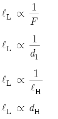
In words, lL is inversely proportional to F, d1, and lH. An increase in F, d1, or lH produces a decrease in lL, and so moves a hole to a higher location on the bore. However, an increase in dH also increases lL and, therefore, moves a hole to a lower location on the bore. A similar analysis indicates the following proportionalities with respect to F:
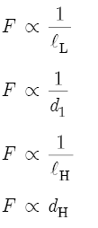
Again in words, F is inversely proportional to lL, d1, and lH, so that increases in these variables produce decreases in F. However, an increase in dH also increases F, which means that after a flute maker has drilled all the tone holes, subtle increases in hole diameter constitute the most important technique for fine-tuning a flute.[42]
[1]Schlesinger, K. (1939). The Greek Aulos, Plate 12 between pp. 74–75, and Plate 17 between pp. 420-421. Methuen & Co. Ltd., London, England.
[2]Nederveen, C.J. (1969). Acoustical Aspects of Woodwind Instruments. Frits Knuf, Amsterdam, Netherlands.
[3]See Appendix B for a complete list of conversion factors.
[4]Acoustical Aspects of Woodwind Instruments, pp. 15–17.
[5]Coltman, J.W. (1979). Acoustical analysis of the Boehm flute. Journal of the Acoustical Society of America 65, No. 2, pp. 499–506.
[6]See Chapter 7, Section 2.
[7]See Chapter 7, Section 11.
[8](a) Acoustical Aspects of Woodwind Instruments, p. 13, pp. 47–48.
(b) Nederveen, C.J. (1973). Blown, passive and calculated resonance frequencies of the flute. Acustica 28, pp. 13–14.
[9]Appendix A lists the frequencies of eight “octaves” in 12-tone equal temperament.
[10]In Figures 8.3(a), 8.3(b), and 8.3(c), the substitution tubes show displacement standing waves with nodes at the ends and an antinode in the center, while the flute tubes show pressure standing waves with nodes at the ends and an antinode in the center. Although such inconsistencies may lead to confusion, here the emphasis is on wavelength and visual imagery and not on wave physics. For a given mode of vibration, a displacement standing wave and a pressure standing wave have exactly the same length.
[11]Benade, A.H., and French, J.W. (1965). Analysis of the flute head joint. Journal of the Acoustical Society of America 37, No. 4, pp. 679–691.
[12]This value assumes no lip coverage at the embouchure hole.
[13]Acoustical Aspects of Woodwind Instruments, p. 26, 47.
With the exception of the key pad correction (ΔlK), Equation 38.8 on p. 64 of Nederveen’s book (or Equation 7 on p. 14 of Nederveen’s article in Acustica 28, 1973) functions as a variable in determining (1) the effective length of the bore at the embouchure hole (as in Equation 8.6 with dE, lE, and d0 variables), and (2) the effective length of the bore at a tone hole (as in Equation 8.14 with dH, lH, and d1 variables). For example, Equation 8.14 is derived in the following manner. On p. 63 of his book, Nederveen gives the outside correction of a tone hole as
![]()
Also on p. 63, Nederveen’s Equation 38.3 is Benade’s solution (see Note 30) for the inside correction of a tone hole. This equation states
The effective length of a tone hole (LH) is then given by
![]()
To use this equation, first simplify Δlin and Δlout:
Now add these two corrections and simplify again:
Therefore, the equivalent effective length of an embouchure hole (LE) equals
This latter equation is more accurate than the denominator of Equation 8.9. Refer to Equation 8.11, and note that a substitution of LH and two equivalent tone hole variables into this equation gives the effective length of the bore at a tone hole location:
A simplification of this equation gives Equation 8.14 in Section 8.5:
And a similar substitution of LE into Equation 8.11 gives Equation 8.6 in Section 8.3:
[14]See Chapter 7.
[15]See Chapter 7, Section 5.
[16]The angular wave number is given by
[17]Richardson, E.G. (1929). The Acoustics of Orchestral Instruments and of the Organ, p. 49, 148. Edward Arnold & Co., London, England.
[18]See Chapter 7, Section 12.
[19]A flute tube three centimeters long has a terminating impedance that is too small for the production of pressure standing waves. In contrast, a tube three meters long has a terminating impedance that is too large for human beings to produce pressure standing waves. Most musicians are not able to deliver the air pressure required for sound production from very long tubes. Furthermore, with respect to tone holes, a very small diameter hole drilled into a flute tube has an extremely large terminating impedance. Pressure waves inside the tube propagate past the tiny hole as though it was not there. Consequently, the presence of such a hole does not change the frequency of the tube.
[20]Benade, A.H. (1976). Fundamentals of Musical Acoustics, p. 449, 495. Dover Publications, Inc., New York, 1990.
Also, see Equation 8.26.
[21]Acustica 28, pp. 12–23.
Nederveen states, “Regarding the outside correction for a hole . . . we observe that the main tube acts as a partial flange to the hole-end, so that we have an end correction in between those for an unflanged end and a fully flanged end.”
[22]Steinkopf, O. (1983). Zur Akustik der Blasinstrumente, p. 19. Moeck Verlag, Celle, Germany.
[23]Acustica 28, 1973, p. 16.
[24](a) Boehm, T. (1847). On the Construction of Flutes, Über den Flötenbau, p. 55. Frits Knuf Buren, Amsterdam, Netherlands, 1982.
The English version of this essay does not have page numbers. A reference to the 50 mm correction in the English translation appears four pages from the end of the book.
(b) Boehm, T. (1871). The Flute and Flute-Playing, p. 42. Dover Publications, Inc., New York, 1964.
Here Boehm gives a slightly longer correction at 51.5 mm.
(c) Fundamentals of Musical Acoustics, p. 495.
[25]This cavity effect is especially significant on concert metal flutes. Here most tone holes have a small chimney that sits above the curved outer surface of the tube. These chimneys provide a straight airtight closing surface for the key pads.
[26]Acoustical Aspects of Woodwind Instruments, p. 76.
[27]Ibid., p. 48.
[28]Ibid., p. 64.
[29]See Note 25.
[30](a) Acoustical Aspects of Woodwind Instruments, p. 64.
(b) Benade, A.H. (1967). Measured end corrections for woodwind toneholes. Journal of the Acoustical Society of America 41, No. 6, p. 1609.
[31]Ibid., p. 48.
[32]See Chapter 9, Section 13.
[33]See Chapter 9, Section 14.
[34]Acoustical Aspects of Woodwind Instruments, p. 48.
[35]Ibid., p. 48, in Figure 32.3.
[36]Rossing, T.D. (1989). The Science of Sound, 2nd ed., pp. 246–247. Addison-Wesley Publishing Co., Inc., Reading, Massachusetts, 1990.
[37]JASA 37, 1965, p. 689.
[38]According to Equation 7.12, a tube open at both ends generates a complete harmonic series of both even-number and odd-number harmonics; and according to Equation 7.17, a tube closed at one end generates an incomplete harmonic series of only odd-number harmonics. The act of overblowing a flute — or increasing the blowing pressure — causes these faint harmonics to sound as plainly audible tones. Therefore, the first overblown tone of a flute open at both ends produces the second harmonic, ratio 2/1; and the first overblown tone of a flute closed at the far end produces the third harmonic, ratio 3/1.
[39]See Chapter 10, Figure 15.
[40]JASA 37, 1965, p. 688.
[41]See Chapter 7, Section 5 through Section 8.
[42]Fundamentals of Musical Acoustics, pp. 473–480.
Another important fine-tuning technique consists of changing the bore diameter of woodwind instruments at the location of a pressure antinode, or at the location of a displacement antinode for a given mode of vibration. If we expand the bore by lightly sanding the inner surface of the flute tube at the location of a pressure antinode, such an increase in diameter causes a local increase in volume (V), which in turn produces a local decrease in pressure. Refer to Equation 7.36, and note that as V increases, the springiness of the air decreases. We may interpret such a local decrease in the air spring constant as causing a decrease in the potential energy of the vibrating system. When the potential energy of a pressure standing wave decreases, the frequency decreases as well. In contrast, if we constrict the bore by applying several coats of lacquer at the location of a pressure antinode, the frequency of a given mode of vibration increases.
On the other hand, a contraction at the location of a displacement antinode decreases the frequency of a given mode of vibration. A local constriction causes an increase in the inertia — or in the resistance to motion — of the air as it flows through the constriction. However, for a given amplitude of vibration, the same volume of air must flow through the constricted portion of the bore per second of time as through the regular bore. This requires an increase in the particle velocity of the air (u) as it passes through the constriction. We may interpret such an increase in particle velocity as causing an increase in the kinetic energy of the vibrating system. When the kinetic energy of a displacement standing wave increases, the frequency decreases. In contrast, if we expand the bore at the location of a displacement antinode, the frequency of a given mode of vibration increases.
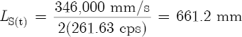
Reminiscent of the discussion in Chapter 6, Section 10, a pattern of overlapping pressure antinodes and displacement antinodes means that a constriction or expansion anywhere along the length of the bore affects numerous modes simultaneously. Moreover, the physical length of a given constriction or expansion also determines which mode frequencies are affected. For example, on the Armstrong flute the constriction of the head joint taper extends 114 mm to the right of the embouchure hole center. Since the embouchure hole marks the location of a displacement antinode of the first mode of vibration, the constriction flattens the frequencies of the first “octave.” Furthermore, according to Chapter 7, Figure 9, a pressure antinode of the second mode of vibration is located a quarter-wavelength (0.25 × λ2) from either end of an open tube. On the Armstrong flute, the C5 pressure antinode exists approximately 115.3 mm to the right of the embouchure hole center. That is, λ2 = c / F2 = 346,000 mm/s ÷ 523.25 cps = 661.3 mm, so that 0.25 × 661.3 mm = 165.3 mm, and 165.3 mm – 50 mm = 115.3 mm. (To locate the position of the second mode pressure antinode with respect to the embouchure hole center, we must account for the embouchure hole correction and, therefore, subtract 50 mm.) Since the 114 mm constriction extends into the vicinity of this pressure antinode, it also sharpens the frequencies of the second “octave.” This sharpening effect on the second register produces tones that are less flat than in the first register. According to Nederveen’s graph in Acustica 28, 1973, p. 17, the head joint taper causes G4 at 392.0 cps to sound 51 cents flat, which gives a frequency of 380.6 cps, and G5 at 784.0 cps to sound only 10 cents flat, which gives a frequency of 779.5 cps. Note, however, that several factors such as increases in the speed of sound due to the warmth and chemical composition of the player’s breath (see Coltman in JASA 40, 1966, pp. 99–107), and increases in the player’s blowing pressure at the embouchure hole, act to sharpen and correct the tendencies of these tones to sound flat. The acoustic need for a tapered head joint is discussed at length by Benade and French in JASA 37, 1965, pp. 679–691, and by Benade in Fundamentals of Musical Acoustics, pp. 495–497.